Continuous Linear Optimal Transport Transform (CLOT)

This tutorial will demonstrate: how to use the forward and inverse operations of the CLOT in the the PyTransKit package.

Class:: CLOT

Continuous Linear Optimal Transport Transform.

Parameters
----------
lr : float (default=0.01)
    Learning rate.
momentum : float (default=0.)
    Nesterov accelerated gradient descent momentum.
decay : float (default=0.)
    Learning rate decay over each update.
max_iter : int (default=300)
    Maximum number of iterations.
tol : float (default=0.001)
    Stop iterating when change in cost function is below this threshold.
verbose : int (default=1)
    Verbosity during optimization. 0=no output, 1=print cost,
    2=print all metrics.

Attributes
-----------
displacements_ : array, shape (2, height, width)
    Displacements u. First index denotes direction: displacements_[0] is
    y-displacements, and displacements_[1] is x-displacements.
transport_map_ : array, shape (2, height, width)
    Transport map f. First index denotes direction: transport_map_[0] is
    y-map, and transport_map_[1] is x-map.
displacements_initial_ : array, shape (2, height, width)
    Initial displacements computed using the method by Haker et al.
transport_map_initial_ : array, shape (2, height, width)
    Initial transport map computed using the method by Haker et al.
cost_ : list of float
    Value of cost function at each iteration.
curl_ : list of float
    Curl at each iteration.

References
----------
[A continuous linear optimal transport approach for pattern analysis in
image datasets]
(https://www.sciencedirect.com/science/article/pii/S0031320315003507)
[Optimal mass transport for registration and warping]
(https://link.springer.com/article/10.1023/B:VISI.0000036836.66311.97)

Functions:

1. Forward transform: lot = forward(sig0, sig1)

   Inputs:
   ----------------
   sig0 : array, shape (height, width)
       Reference image.
   sig1 : array, shape (height, width)
       Signal to transform.
   
   Outputs:
   ----------------
   lot : array, shape (2, height, width)
       LOT transform of input image sig1. First index denotes direction:
       lot[0] is y-LOT, and lot[1] is x-LOT.
   

2. Apply forward transport map: sig0_recon = apply_forward_map(transport_map, sig1)

   Inputs:
   ----------------
   transport_map : array, shape (2, height, width)
       Forward transport map.
   sig1 : array, shape (height, width)
       Signal to transform.
   
   Outputs:
   ----------------
   sig0_recon : array, shape (height, width)
       Reconstructed reference signal sig0.
   

3. Apply inverse transport map: sig1_recon = inverse(transport_map, sig0)

   Inputs:
   ----------------
   transport_map : array, shape (2, height, width)
       Forward transport map. Inverse is computed in this function.
   sig0 : array, shape (height, width)
       Reference signal.
   
   Outputs:
   ----------------
   sig1_recon : array, shape (height, width)
       Reconstructed signal sig1.
   

Definition

The Continuous Linear Optimal Transport (CLOT) transform \(\widehat s\) of a density function \(s(\mathbf x)\) is defined as the optimal transport map from a reference density \(s_0(\mathbf x)\) to \(s(\mathbf x)\). Specifically, let \(s_0(\mathbf x), s(\mathbf x)\) be positive functions defined on domains \(\Omega_{s_0}, \Omega_{s}\subseteq \mathbb R^d\) respectively and such that

\[\int_{\Omega_{s_0}}s_0(\mathbf x) d\mathbf x = \int_{\Omega_{s}}s(\mathbf x) d\mathbf x =1 \quad \text{(normalized)}.\]

Assuming that the density functions \(s_0, s\) have finite second moments, there is an unique solution to the Monge optimal transport problem:

\begin{align} \label{Monge} &\text{min Monge }(T)=\int_{R^d}\big|x-T(x)\big|^2s_0(x)dx, \qquad (1)\\ &\text{s.t.}\quad \int_{B}s(\mathbf y)d\mathbf y= \int_{T^{-1}(B)} s_0(\mathbf x) d\mathbf x, \quad \text{for all open} \ B\subseteq \mathbb R^d. \qquad (2) \label{mass-preserving} \end{align}

Any map \(T\) satisfying constraint in (2) is called a transport (mass-preserving) map between \(s_0\) and \(s\). In particular, when \(T\) is bijective and continuously differentiable, the mass-preserving constraint in (2) becomes

\begin{equation} \label{MassCons} s_0(x)= \big|\det \big(\nabla T(x)\big)\big|s\big(T(x)\big). \end{equation}

The minimizer to the above Monge problem is called an optimal transport map. Given a fixed reference density \(s_0\), the LOT transform \(\widehat s\) of a density function \(s\) is defined to the unique optimal transport map from \(s_0\) to \(s\). Moreover Brenier [1] shows that any optimal transport map can be written as the gradient of a convex function, i.e., \(\widehat s = \nabla \phi\) where \(\phi\) is a convex function. Following the generic approach described in [2], Kolouri et al. [3] employed an iterative algorithm minimizing (1) with constraint (2) via the gradient descent idea.

References

[1] Y. Brenier. Polar factorization and monotone rearrangement of vector-valuedfunctions.Commun. Pure Appl. Math., 44(4):375–417, 1991.1 [2] S. Haker, L. Zhu, A. Tannenbaum, and S. Angenent. Optimal mass transport forregistration and warping.Int. J. Comput. Vis., 60(4):225–240, 2004. [3] S. Kolouri, A. Tosun, J. Ozolek, and G. Rohde. A continuous linear optimal trans-port approach for pattern analysis in image datasets.Pattern Recognit., 51:453–462, 2016.

CLOT Demo

The examples will cover the following operations: * Forward operation of the CLOT * Apply forward map to transport \(I_1\) to \(I_0\) * Apply inverse map to reconstruct \(I_1\) from \(I_0\)

Forward CLOT

Import necessary python packages

import numpy as np
import matplotlib.pyplot as plt

Read and normalize two images \(I_0\) and \(I_1\).

import matplotlib.image as mpimg
import sys
sys.path.append('../')
from pytranskit.optrans.utils import signal_to_pdf

I0 = mpimg.imread('images/I0.bmp')
I1 = mpimg.imread('images/I1.bmp')

# Convert images to PDFs
img0 = signal_to_pdf(I0, sigma=1., total=100.)
img1 = signal_to_pdf(I1, sigma=1., total=100.)

fig, ax = plt.subplots(1, 2, sharex=True, sharey=True, figsize=(5,10))
ax[0].imshow(img0,cmap='gray')
ax[1].imshow(img1,cmap='gray')
ax[0].set_title('$I_0$')
ax[1].set_title('$I_1$')
ax[0].axis('off')
ax[1].axis('off')
plt.show()

Compute CLOT and apply forward map

from pytranskit.optrans.continuous.clot import CLOT
from pytranskit.optrans.utils import plot_displacements2d

clot = CLOT(max_iter=500, lr=1e-6, tol=1e-4,verbose=0)

# calculate CLOT
lot = clot.forward(img0, img1)

# transport map and displacement map from I1 to I0
tmap10 = clot.transport_map_
disp = clot.displacements_

# apply forward map to transport I1 to I0
img0_recon = clot.apply_forward_map(tmap10, img1)

fig, ax = plt.subplots(1, 4, sharex=True, sharey=True, figsize=(10,20))
ax[0].imshow(img0, cmap='gray')
ax[0].set_title('$I_0$')

ax[1].imshow(img1, cmap='gray')
ax[1].set_title('$I_1$')

ax[2].imshow(img0_recon, cmap='gray')
ax[2].set_title('$f^{\'}I_1\circ f$')

plot_displacements2d(disp, ax=ax[3], count=20)
ax[3].set_title('Displacement')

plt.show()

Inverse CLOT

Apply inverse map on \(I_0\) to reconstruct \(I_1\)

img1_recon = clot.apply_inverse_map(tmap10, img0)

fig, ax = plt.subplots(1, 3, sharex=True, sharey=True, figsize=(8,15))
ax[0].imshow(img1, cmap='gray')
ax[0].set_title('$I_1$')

ax[1].imshow(img0, cmap='gray')
ax[1].set_title('$I_0$')

ax[2].imshow(img1_recon, cmap='gray')
ax[2].set_title('$(f^{-1})\'I_0\circ f^{-1}$')

ax[0].axis('off')
ax[1].axis('off')
ax[2].axis('off')

plt.show()

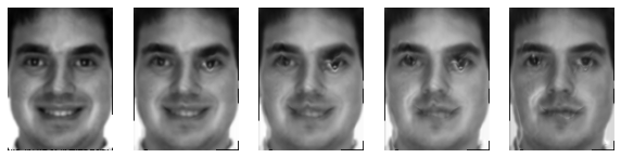
Geodesic

Show points on the geodesic between \(I_0\) and \(I_1\)

lot11 = clot.forward(img1, img1)
tmap11 = clot.transport_map_

alpha = np.linspace(0,1,5)
img_recon = []
fig, ax = plt.subplots(1, len(alpha), sharex=True, sharey=True, figsize=(10,5*len(alpha)))
for i in range(len(alpha)):
    tmap = alpha[i]*tmap10 + (1-alpha[i])*tmap11
    img_recon.append(clot.apply_forward_map(tmap, img1))
    ax[i].imshow(img_recon[i],cmap='gray')
    ax[i].axis('off')
plt.show

<function matplotlib.pyplot.show(*args, **kw)>