3D Radon-Cumulative Distribution Transform (3D R-CDT)

This tutorial will demonstrate: how to use the forward and inverse operations of the 3D R-CDT in the PyTransKit package.

Class:: RadonCDT3D

Parameters:

Npoints : scaler, number of radon projections (default = 1024)
use_gpu : boolean, use GPU if True (default = False)

Functions:

1. Forward transform: sig1_hat = forward(x0_range, sig0, x1_range, sig1)

   Inputs:
   ----------------
   x0_range : 1x2 array
       contains lower and upper limits for independent variable of reference signal (sig0). Example: [0,1].
   sig0 : 3d array, shape (L, L, L)
       Reference signal.
   x1_range : 1x2 array
       contains lower and upper limits for independent variable of input signal (sig1). Example: [0,1].
   sig1 : 3d array, shape (L, L, L)
       Signal to transform.
   
   Outputs:
   ----------------
   sig1_hat : 2d array, shape(L, Npoints)
       R-CDT of 3D input signal sig1.
   

2. Inverse transform: sig1_recon = inverse(sig1_hat, sig0, x1_range)

   Inputs:
   ----------------
   sig1_hat : 2d array, shape(L, Npoints)
       R-CDT of 3D signal sig1.
   sig0 : 3d array, shape (L, L, L)
       Reference signal.
   x1_range : 1x2 array
       contains lower and upper limits for independent variable of input signal (sig1). Example: [0,1].
   
   Outputs:
   ----------------
   sig1_recon : 3d array, shape (L, L, L)
       Reconstructed signal.
   

Example

The example will cover the following operations: * Forward and inverse operations of the 3D R-CDT

import sys
sys.path.append('../')
from pytranskit.optrans.continuous.radoncdt3D import RadonCDT3D

import time
import numpy as np
from scipy.io import loadmat
import matplotlib.pyplot as plt
%matplotlib inline

Forward 3D Radon-CDT

Load 3D phantom data from ‘images/’ direcotry

datafile = 'images/phantom3D.mat'
img3D = loadmat(datafile)['phantom3D']
i03D = np.ones(img3D.shape)

Run forward 3D R-CDT on the 3D phantom data

use_gpu = False  # Set it True if want GPU support
x0_range = [0,1]
x_range = [0,1]
Npoints = 1000

# Create an instance of 3D R-CDT
rcdt3D = RadonCDT3D(Npoints, use_gpu)

tic=time.time()
# Forward function
img3Dhat=rcdt3D.forward(x0_range, i03D/np.sum(img3D), x_range, img3D/np.sum(img3D), rm_edge=False)

toc=time.time()
Run_time = toc - tic
print("Forward 3D RCDT is done in {} seconds".format(Run_time))

Forward 3D RCDT is done in 19.50796389579773 seconds

Inverse 3D Radon-CDT

tic=time.time()
# Inverse function
img3D_recon = rcdt3D.inverse(img3Dhat, i03D, x_range)
toc=time.time()
Run_time = toc - tic
print("Inverse 3D RCDT is done in {} seconds".format(Run_time))

Inverse 3D RCDT is done in 20.88492465019226 seconds

Show results

Show specific slices from the input 3D phantom image and reconstructed image

sliceSel = int(0.5*img3D.shape[0])

# plot original 3D image
plt.figure(figsize=(15,5))
plt.suptitle('3D Phantom')
plt.subplot(131)
plt.imshow(img3D[sliceSel,:,:])
plt.title('Axial view')

plt.subplot(132)
plt.imshow(img3D[:,sliceSel,:])
plt.title('Coronal view')

plt.subplot(133)
plt.imshow(img3D[:,:,sliceSel])
plt.title('Sagittal view')
plt.show()

# plot 3D Radon transform
fig=plt.figure(figsize=(15,5))
plt.imshow(img3Dhat)
plt.title('3D R-CDT')
plt.show()

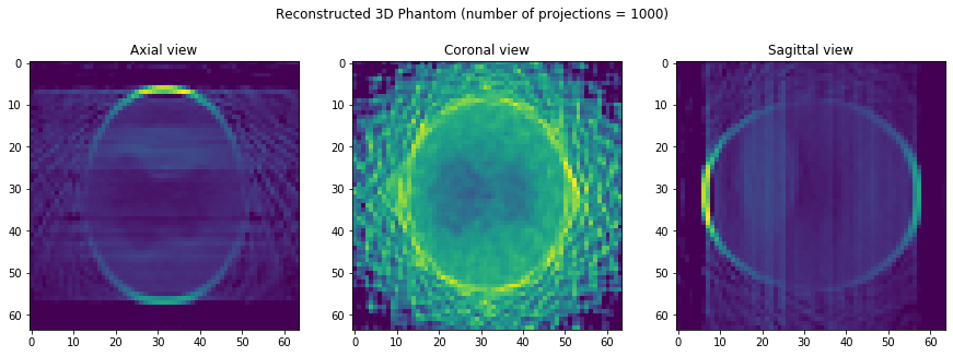
# plot 3D reconstruction
plt.figure(figsize=(15,5))
plt.suptitle('Reconstructed 3D Phantom (number of projections = {})'.format(Npoints))
plt.subplot(131)
plt.imshow(np.log10(.1+img3D_recon[sliceSel,:,:]))
plt.title('Axial view')

plt.subplot(132)
plt.imshow(np.log10(.1+img3D_recon[:,sliceSel,:]))
plt.title('Coronal view')

plt.subplot(133)
plt.imshow(np.log10(.1+img3D_recon[:,:,sliceSel]))
plt.title('Sagittal view')
plt.show()